Selecting the right blower by understanding air flow

For engineers tired of guessing their way through blower selection, this white paper cuts through the noise with a clear, methodical framework. It walks you from operating point and system resistance curves through the fan laws and density corrections that actually matter when your prototype does not hit its numbers, and is the kind of practical reference you will come back to every time you’re staring down a spec sheet wondering which curve is the right one

Selecting a blower for a particular application first requires knowledge or an estimate of the application’s operating point: the flow rate required and the resistance to flow that the system, ductwork, filters, and other obstructions will impose.

 This resistance creates a loss of static pressure in the flow system, often referred to as backpressure or head loss, and each blower has a characteristic curve that describes the maximum amount of resistance that it can overcome to provide a given flow rate.

Manufacturer performance curves represent each model’s typical maximum performance (full speed) at a constant input voltage. The performance curve describes a blower’s ability to deliver flow rate through resistance — from zero backpressure (‘open flow’) to completely blocked flow (‘sealed’). Since all BLDC blowers have adjustable speed control, any operating point that lies underneath a given performance curve can be reached, although there are several factors to consider beyond this.

With knowledge of the desired operating point, it is then a simple matter to identify blowers having performance curves that meet or exceed the desired operating point. Other factors should then be considered, which will be discussed below.

System resistance curve

A resistance to flow is typically characterised by a static pressure drop for a given flow rate, and often follows a 2nd order relationship (see Figure 1).

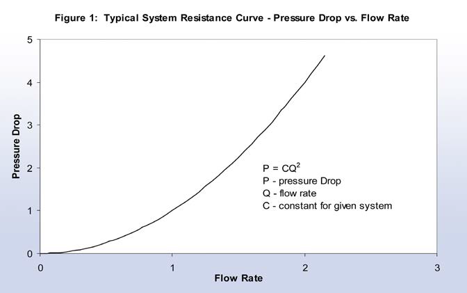
(in some cases such as certain filters, the relationship is more linear). If the desired operating point is known, then its associated system curve can be estimated according to the relationship P=CQ2. 

Plugging the values for desired operating point into the P (pressure drop) and Q (flow rate) terms yields the constant C. The system curve can then be overlaid graphically onto a given blower performance curve. 

The intersection of the two curves is the actual operating point (see Figure 2).

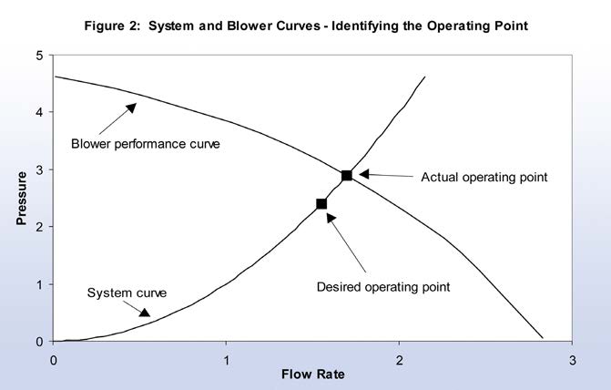
The static pressure rise provided by the blower matches the static pressure loss imposed by the system resistance. For quick checks, simply place the operating point on a given blower curve and ‘eyeball’ the system curve through it.

There are likely to be several models that can achieve an application’s performance requirement for flow rate and static pressure, but not all will necessarily operate with the same efficiency. Blower performance curves include not only static pressure vs. flow rate information, but also current, rotational speed, and input power vs. flow rate. 

An application is normally best served by selecting the blower that delivers the desired performance with the best efficiency, i.e., the least amount of input power. For quick comparisons, a blower’s peak efficiency lies near the middle of the flow range (i.e., about half the maximum flow rate) so it is recommended to look for blowers that have curves that intersect the system curve in the middle region rather than near the open flow or sealed points.

Other questions to consider when selecting a blower:

• What are the size constraints for fitting into my application?
• Would I prefer that the blower have an on-board brushless DC controller or would I prefer to provide an external controller?
• Do I need a blower with fast dynamic response?
• Is loudness a major factor?
• Does my application require modulating the speed during operation or simply a single speed adjustment made at the time of installation?
• What input voltage will I have available for powering the blower?
• Are there additional features that I require such as a tachometer output, dynamic braking, or speed control functions?
• Is it a problem for the working fluid to come into contact with electronics?
• What are the environmental factors associated with my application?

Blower performance vs. speed change

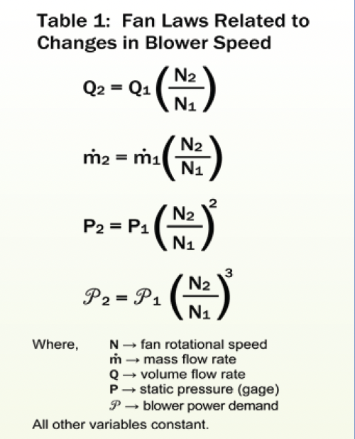
Since BLDC blowers are speed controllable, the speed can be reduced to a desired operating point or increased if a different operating point is needed in a dynamic system. Blowers conveniently have very predictable behavior when it comes to changes in speed. Table 1 summarises these relationships. Figure 3 with Example 1 demonstrates how to calculate the power requirement for an operating point that occurs at a reduced speed.

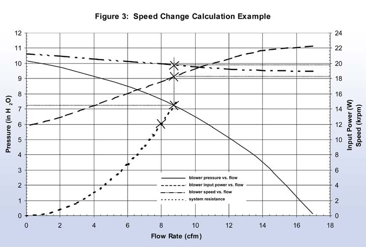
Example 1: An application calls for air performance of 8 cfm (ft3/min) at a static pressure of 6 inch H2O. The blower whose performance is shown in Figure 3 has been chosen. What will be the power consumption at 8cfm, 6 in H2O?

Answer: At full speed, the blower will deliver about 8.8 cfm in this system, whose static pressure loss is about 7.2 in H2 O at that flow rate (see Figure 3). Since this is delivering too much flow rate, the speed must be reduced to achieve the desired operating point. At full speed, Figure 3 shows the blower speed to be about 19. kprm and the power consumption is 18.3W. Using the fan laws shown in Table 1 yields:  

  = 18.0 krpm

So, the power consumption at the reduced speed is:  

The speed at the desired operating point could also have been found by using the ratio of pressures:  

Note: There is some minor error in this calculation because there will likely be some small change in motor efficiency at the different operating points. This can usually be neglected for estimating power requirements.

Fluid density

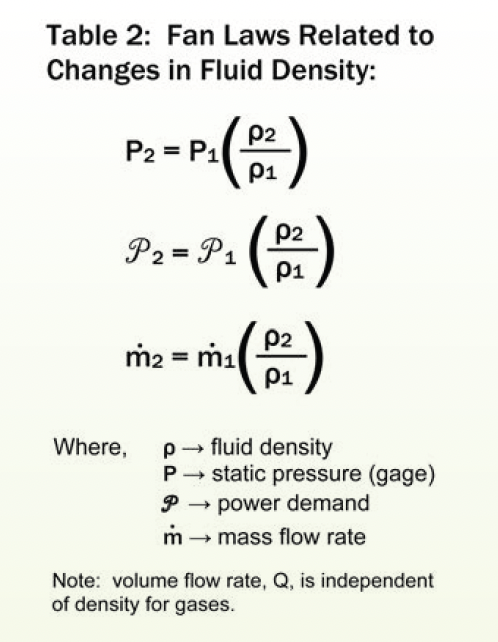
The density of the working fluid has a significant influence on blower performance, as can be seen in the relationships listed in Table 2. Because fluid density is a variable that is independent of the blower, the density must be stated as part of any blower performance specification. In the previous example, the density was ignored for simplicity. But the performance curves for most blowers have the statement ‘corrected to density = .075lb/ft3’ , or equivalent statement. So, in the previous example, it was assumed that the desired performance of (8 cfm, 6 in H2 O) had also been corrected to .075 lb/ft3 . The density value of .075 lb/ft3 is a somewhat arbitrary selection, but it is close to typical air density at sea level. It is commonly referred to as “Standard Density” in the fan and blower industry. Any target operating point must be corrected to .075 lb/ft3 when evaluating blower performance curves. Examples hereafter demonstrate how to do this.

The vast majority of blower applications are designed to move air, but blowers can be used with any nonexplosive, non-corrosive gas mixture (Note: some specialised blowers are designed for combustion pre-mix applications). At the temperature and pressure ranges for most blower applications, the gas mixture can be considered an ideal gas, and it will behave according to the relationship:  

Where, 

P = the absolute pressure

ρ = the density

Ru = the universal gas constant

T = the absolute temperature

M = the molar mass

For gas mixtures, the molar mass of the mixture can be determined from the weighted average of the component gases. 

Air density

 Determining air density requires knowing the temperature, barometric pressure, and humidity of the working environment. Measuring temperature is relatively easy, but barometric pressure requires a barometer, and humidity requires either a wet bulb thermometer, a hygrometer, or a dew point detector. (Note: be careful if using barometric values obtained from weather services — they are corrected for altitude and may not match an actual on-site barometer measurement.)

Once these values are known, the easiest way to determine density is to use a psychrometric chart, which gives the properties of air for large ranges of temperature and humidity. (There are also online calculators available). Some notes on using a psychrometric chart:

1) Instead of density, the specific volume, which is the reciprocal of density, usually is plotted.

2) The specific volume is typically given in terms of volume per unit mass of dry air. But the working fluid is a mixture of air and water vapor (except at 0% humidity, of course). See the example hereafter for calculating the actual specific volume, i.e., volume per unit mass of the air-water vapor mixture.

3) Dry bulb temperature is simply the temperature measured using a regular thermometer.

4) For humidity, the wet bulb temperature can be used directly without having to convert to another type of humidity quantity. As an alternative, relative humidity or humidity ratio can be used.

5) Psychrometric charts are plotted at a single barometric pressure which is noted in the heading of the chart. A correction is needed to adjust density values to the actual barometric pressure.

Example 2: A laboratory makes the following measurements of the ambient air conditions:

Barometric pressure = 28.60 in Hg

Dry bulb temperature = 72° F

Wet bulb temperature = 65° F

What is the ambient density?

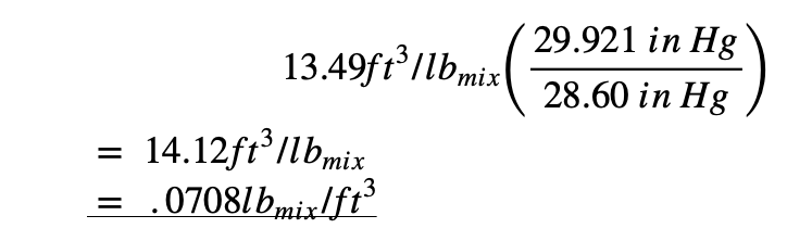
Answer: Using a psychrometric chart plotted at 29.921 in Hg, the intersections of the curves corresponding to the dry bulb and wet bulb values above yields a specific volume of 13.64ft3/lb

dry air and a humidity ratio of .0116  per. Correct the specific volume per lb air-water vapour mixture:

Finally, correcting this value for the actual barometric pressure yields:  

The density of air varies substantially with weather and altitude. The Standard Atmosphere Table (not included herein, but widely available in reference texts and internet sites) gives a good estimate for typical outdoor ambient conditions as a function of altitude. The following example demonstrates how to account for the lower density at high altitude:

Example 3: An application calls for a blower to deliver 50cfm of air at 30 inch H2O at an altitude of 7000ft above sea level where the average air density is 0.062 lb/ft3, according to the Standard Atmosphere Table. For the purpose of selecting a blower, what operating point should be used?

Answer: Refer to Table 2. Since volume flow rate does not change with density, the flow rate remains at 50 cfm. The pressure does change in proportion to density: 

So, the operating point corrected to standard density is 50cfm, 36.3 inch .

Example 3 continued: A blower is selected that can deliver the above performance with a power demand of 600 W at standard density, as shown on the performance curves. What will be the

power demand at the intended location at 7000ft altitude?

Answer: Refer to Table 2 for correcting power demand for a change in density. 

Example 3 continued — Redefining the problem in terms of mass flow rate: The application requires a mass flow rate of 3.1 lb/min of air regardless of altitude.

How much must the speed be reduced if the application is moved from a location at 7000ft (.062 lb/ft3) to sea level (.075 lb/ft3)?

Answer: Table 2 shows that the change in mass flow rate is a simple ratio of the densities. If the blower speed is maintained between the two locations, the mass flow rate delivered at sea level will be:

Mass flow rate is directly proportional to a change in speed (Table 1), so to maintain 3.1 lb/ft³, the speed must be reduced by:

3.10 lb/min=3.75 lb/min(N2/N1)

(N2/N1)=.827=17.3% reduction

How much will the power demand change?

Answer: Tables 1 and 2 show that the power demand is directly proportional to both density and speed, although a speed change has a much larger influence. Combining both relationships yields: 

Selecting the right blower starts with clearly defining the required operating point, then matching that requirement to manufacturer performance curves and the system resistance curve so the actual flow and pressure needs are met efficiently. By understanding how speed changes, fan laws, and fluid density affect flow, pressure, and power demand, engineers can accurately predict performance across different operating conditions and environments. Considering additional factors such as control method, noise, physical constraints, and environmental conditions further ensures that the chosen blower delivers reliable, optimised performance over its service life.

For more information, visit Bison.